Routing problems¶

Todo

Adapt everything: figures, maths, …

In this chapter we will consider several problems related to routing, discussing and characterizing different mathematical optimization formulations. The roadmap is the following. Section Traveling Salesman Problem presents several mathematical formulations for the traveling salesman problem (TSP), one of the most extensively studied optimization problems in operations research. In section Traveling Salesman Problem with Time Windows we extend one of the formulations for the TSP for dealing with the case where there is a time interval within which each vertex must be visited. Section Capacitated Vehicle Routing Problem describes the capacity-constrained delivery planning problem, showing a solution based on the cutting plane method.

Traveling Salesman Problem¶

Here we consider the traveling salesman problem, which is a typical example of a combinatorial optimization problem in routing. Let us start with an example of the traveling salesman problem.

You are thinking about taking a vacation and taking a tour of Europe. You are currently in Zurich, Switzerland, and your aim is to watch a bullfight in Madrid, Spain, to see the Big Ben in London, U.K., to visit the Colosseum in Rome, Italy, and to drink authentic beers in Berlin, Germany. You decide to borrow a rental helicopter, but you have to pay a high rental fee proportional to the distance traveled. Therefore, after leaving, you wish to return to Zurich again, after visiting the other four cities (Madrid, London, Rome, Berlin) by traveling a distance as short as possible. Checking the travel distance between cities, you found that it is as shown in Figure Traveling salesman problem. Now, in what order should you travel so that distance is minimized?

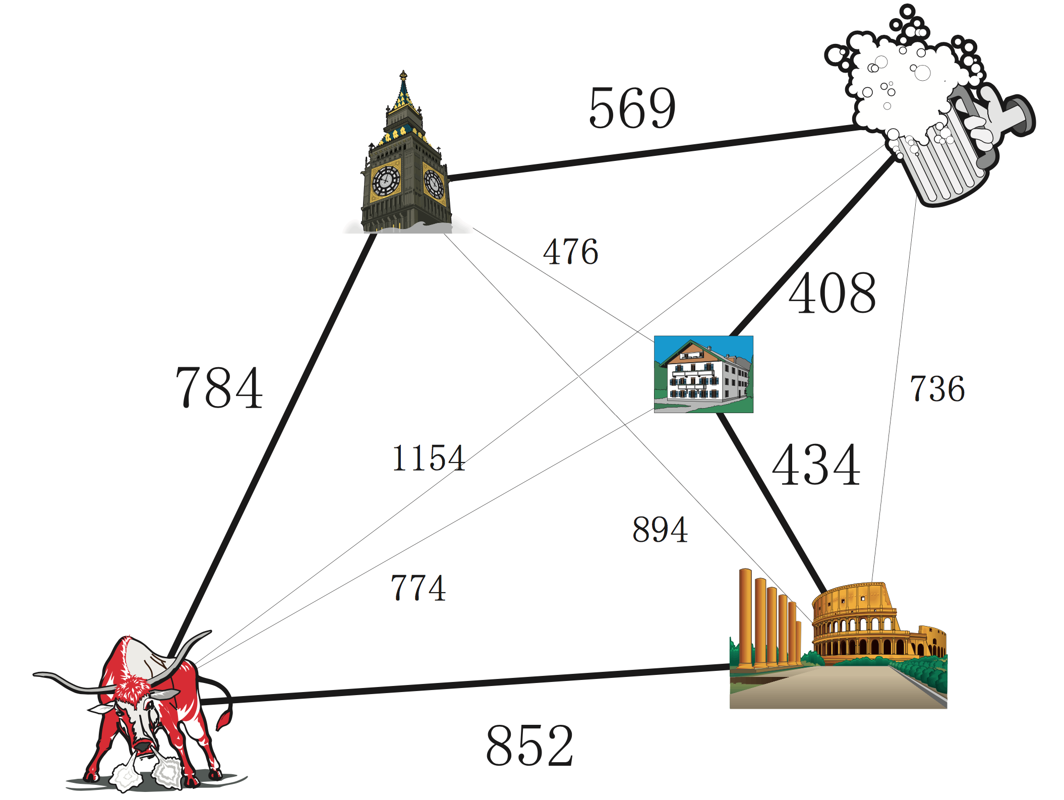
Traveling salesman problem

Graph representation of cities in Europe (numerical value on edirs is the distance in miles) and optimum solution (thick line).

Let us define the problem without ambiguity. This definition is based on the concept of graph, introduced in Section Graph problems.

Traveling salesman problem (TSP)

Given an undirected graph $G = (V, E)$ consisting of $n$ vertices (cities), a function $c: E \to \mathbb{R}$ associating a distance (weight, cost, travel time) to each edge, find a tour which passes exactly once in each city and minimizes the total distance (i.e., the length of the tour).

When the problem is defined on a non-oriented graph (called an undirected graph), as in the above example, we call it a symmetric traveling salesman problem. Symmetric means that the distance from a given point $a$ to another point $b$ is the same as the distance from $b$ to $a$. Also, the problem defined on a graph with orientation (called a directed graph or digraph)) is called an asymmetric traveling salesman problem; in this case, the distance for going from a point to another may be different of the returning distance. Of course, since the symmetric traveling salesman problem is a special form of the asymmetric case, a formulation for the latter can be applied as it is to symmetric problems (independently from whether it can be solved efficiently or not).

In this section we will see several formulations for the traveling salesman problem (symmetric and asymmetric) and compare them experimentally. Section Subtour elimination formulation presents the subtour elimination formulation for the symmetric problem proposed by Dantzig-Fulkerson-Johnson [DFJ54]. Section Miller-Tucker-Zemlin (potential) formulation presents an enhanced formulation based on the notion of potential for the asymmetric traveling salesman problem proposed by Miller-Tucker-Zemlin [MTZ69]. Sections Single-commodity flow formulation and Multi-commodity flow formulation propose formulations using the concept of flow in a graph. In Single-commodity flow formulation we present a single-commodity flow formulation, and in Multi-commodity flow formulation we develop a multi-product flow formulation.

Subtour elimination formulation¶

There are several ways to formulate the traveling salesman problem. We will start with a formulation for the symmetric case. Let variables $x_e$ represent the edges selected for the tour, i.e., let $x_e$ be 1 when edge $e \in E$ is in the tour, 0 otherwise.

For a subset $S$ of vertices, we denote $E(S)$ as the set of edges whose endpoints are both included in $S$, and $\delta(S)$ as the set of edges such that one of the endpoints is included in $S$ and the other is not. In order to have a traveling route, the number of selected edges connected to each vertex must be two. Besides, the salesman must pass through all the cities; this means that any tour which does not visit all the vertices in set $V$ must be prohibited. One possibility for ensuring this is to require that for any proper subset $S \subset V$ with cardinality $|S| \geq 2$, the number of selected edges whose endpoints are both in $S$ is, at most, equal to the number of vertices $|S|$ minus one.

From the above discussion, we can derive the following formulation.

\[\begin{split}& \mbox{minimize} \quad & \sum_{e \in E} c_{e} x_{e} & \\ & \mbox{subject to} \quad & \sum_{e \in \delta(\{i\})} x_{e} = 2 \qquad & \forall i \in V,\\ & & \sum_{e \in E(S)} x_{e} \leq |S|-1 \qquad & \forall S \subset V, 2 \leq |S| \leq |V|-2,\\ & & X_{e} \in \{0,1\} & \forall e \in E.\end{split}\]

Since the number of edges connected to a vertex is called its degree, the first constraint is called degree constraint. The second constraint is called the subtour elimination inequality because it excludes partial tours (i.e., cycles which pass through a proper subset of vertices; valid cycles must pass through all the vertices).

For a given subset $S$ of vertices, if we double both sides of the subtour elimination inequality and then subtract the degree constraint

\[\sum_{e \in \delta(\{i\})} x_{e} = 2\]

for each vertex $i \in S$, we obtain the following inequality:

\[\begin{split}\sum_{e \in \delta(S)} x_{e} \geq 2, \qquad & \forall S \subset V, |S| \geq 2. \\\end{split}\]

This constraint is called a cutset inequality, and in the case of the traveling salesman problem it has the same strength as the subtour elimination inequality. In the remainder of this chapter, we consider only the cutset inequality.

The number of subsets of a set increases exponentially with the size of the set. Similarly, the number of subtour elimination constraints (cutset constraints) for any moderate size instance is extremely large. Therefore, we cannot afford solving the complete model; we have to resort to the so-called cutting plane method, where constraints are added as necessary.

Assuming that the solution of the linear relaxation of the problem using only a subset of constraints is $\bar{x}$, the problem of finding a constraint that is not satisfied for this solution is usually called the separation problem (notice that components of $\bar{x}$ can be fractional values, not necessarily 0 or 1). In order to design a cutting plane method, it is necessary to have an efficient algorithm for the separation problem. In the case of the symmetric traveling salesman problem, we can obtain a violated cutset constraint (a subtour elimination inequality) by solving a maximum flow problem for a network having $\bar{x}_e$ as the capacity, where $\bar{x}_e$ is the solution of the linear relaxation with a (possibly empty) subset of subtour elimination constraints. Notice that if this solution has, e.g., two subtours, the maximum flow from any vertex in the first subtour to any vertex in the second is zero. By solving finding the maximum flow problem, we also obtain the solution of the minimum cut problem, i.e., a partition of the set of vertices $V$ into two subsets $(S, V \setminus S)$ such that the capacity of the edges between $S$ and $V \setminus S$ is minimum [FF56]. A minimum cut is obtained by solving the following max-flow problem, for sink vertex $k = 2, 3, \ldots, n$:

\[\begin{split}\mbox{maximize} \quad & \sum_{j: j>1} f_{1j} & \\ \mbox{subject to} \quad & \sum_{j: i<j} f_{ij} - \sum_{j: i>j} f_{ji} = 0 \qquad & \forall i : i \neq 1, i \neq k \\ & -\bar{x}_{ij} \leq f_{ij} \leq \bar{x}_{ij} \qquad & \forall i < j\end{split}\]

The objective represents the total flow out of node 1. The first constraint concerns flow preservation at each vertex other than the source vertex 1 and the target vertex $k$, and the second constraint limits flow capacity on each arc. In this model, in order to solve a problem defined on an undirected graph into a directed graph, a negative flow represents a flow in the opposite direction.

As we have seen, if the optimum value of this problem is less than 2, then a cutset constraint (eliminating a subtour) which is not satisfied by the solution of the previous relaxation has been found. We can determine the corresponding cut $(S, V \setminus S)$ by setting $S = \{ i \in V : \pi_i \neq 0 \}$, where $\pi$ is the optimal dual variable for the flow conservation constraint.

Here, instead of solving the maximum flow problem, we will use a convenient method to find connected components for the graph consisting of the edges for which $x_e$ is positive in the previous formulation, when relaxing part of the subtour elimitation constraints. A graph is said to be connected if there is a path between any pair of its vertices. A connected component is a maximal connected subgraph, i.e., a connected subgraph such that no other connected subgraph strictly contains it. To decompose the graph into connected components, we use a Python module called networkX [1].

The following function addcut takes as argument a set of edges, and can be used to add a subtour elimination constraint corresponding to a connected component $S (\neq V)$.

 def addcut(cut_edges):
     G = networkx.Graph()
     G.add_edges_from(cut_edges)
     Components = list(networkx.connected_components(G))
     if len(Components) == 1:
         return False
     model.freeTransform()
     for S in Components:
         model.addCons(quicksum(x[i,j] for i in S for j in S if j>i) <= len(S)-1)
     return True

In the second line of the above program, we create an empty undirected graph object $G$ by using the networkx module and construct the graph, by adding vertices and edges in the current solution cut_edges, in line 3. Next, in line 4, connected components are found by using function connected_components. If there is one connected component (meaning that there are no subtours), False is returned. Otherwise, the subtour elimination constraint is added to the model (lines 7 to 10).

Using the addcut function created above, an algorithm implementing the cutting plane method for the symmetric travelling salesman problem is described as follows.

 def solve_tsp(V,c):
     model = Model("tsp")
     model.hideOutput()
     x = {}
     for i in V:
         for j in V:
             if j > i:
                 x[i,j] = model.addVar(ub=1, name="x(%s,%s)"%(i,j))
     for i in V:
         model.addCons(quicksum(x[j,i] for j in V if j < i) + \
                       quicksum(x[i,j] for j in V if j > i) == 2, "Degree(%s)"%i)
     model.setObjective(quicksum(c[i,j]*x[i,j] for i in V for j in V if j > i), "minimize")
     EPS = 1.e-6
     isMIP = False
     while True:
         model.optimize()
         edges = []
         for (i,j) in x:
             if model.getVal(x[i,j]) > EPS:
                 edges.append( (i,j) )
         if addcut(edges) == False:
             if isMIP:     # integer variables, components connected: solution found
                 break
             model.freeTransform()
             for (i,j) in x:     # all components connected, switch to integer model
                 model.chgVarType(x[i,j], "B")
                 isMIP = True
     return model.getObjVal(),edges

Firstly, the linear optimization relaxation of problem (without subtour elimination constraints) is constructed from lines 4 to 12. Next, in the while iteration starting at line 15, the current model is solved and cut constraints are added until the number of connected components of the graph becomes one. When there is only one connected component, variables are restricted to be binary (lines 25 and 26) and the subtour elimination iteration proceeds. When there is only one connected component in the problem with integer variables, it means that the optimal solution has been obtained; therefore the iteration is terminated and the optimal solution is returned.

In the method described above, we used a method to re-solve the mixed integer optimization problem every time a subtour elimination constraint is added. However, it is also possible to add these constraints during the execution of the branch-and-bound process.

!!!!! How, in SCIP ????? ..

but applying the branch and bound method by using the cbLazy function added in Gurobi 5.0

Note

Margin seminar 6

Cutting plane and branch-and-cut methods

The cutting plane method was originally applied to the traveling salesman problem by George Dantzig, one of the founders of linear optimization, and his colleagues Ray Fulkerson and Selmer Johnson, in 1954. Here, let us explain it by taking as an example the maximum stable set problem, introduced in Section mssp.

Let’s consider a simple illustration consisting of three points (Figure Polyhedra for the maximum stable set problem, top). Binary variables $x_1, x_2, x_3$, represented as a point in the three-dimensional space $(x_1, x_2, x_3)$, indicate whether the corresponding vertices are in the maximum stable set or not. Using these variables, the stable set problem can be formulated as an integer optimization problem as follows.

\[\begin{split}& \mbox{maximize} \quad & x_1 + x_2 + x_3\\ & \mbox{subject to} \quad & x_1 + x_2 \leq 1\\ & & x_1 + x_3 \leq 1\\ & & x_2 + x_3 \leq 1\\ & & x_1, x_2, x_3 \in \{0,1\}\end{split}\]

The constraints in the above formulation state that both endpoints of an edge can not be placed in a stable set at the same time. This instance has four feasible solutions: $(0,0,0), (1,0,0), (0,1,0), (0,0,1)$. The smallest space that “wraps around” those points is called a polytope; in this case, it is a tetrahedron, defined by these 4 points, and shown in the bottom-left image of Figure Polyhedra for the maximum stable set problem. An optimal solution of the linear relaxation can be obtained by finding a vertex of the polyhedron that maximizes the objective function $x_1 + x_2 + x_3$. This example is obvious, and any of the points $(1, 0, 0), (0, 1, 0), (0, 0, 1),$ is an optimal solution, with optimum value 1.

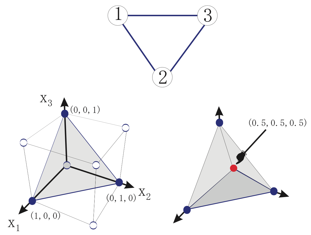
Polyhedra for the maximum stable set problem

Maximum stable set instance (upper figure). Representation of the feasible region as a polyhedron, based on its extreme points (lower-left figure). The inequality system corresponding to its linear relaxation is is $x_1 + x_2 \leq 1; x_1 + x_3 \leq 1; x_2 + x_3 ≤ 1; x_1, x_2, x_3 ≥ 0$; this space, and an optimum solution, are represented in the lower-right figure.

In general, finding a linear inequality system to represent a polyhedron — the so-called convex envelope of the feasible region — is more difficult than solving the original problem, because all the vertices of that region have to be enumerated; this is usually intractable. As a realistic approach, we will consider below a method of gradually approaching the convex envelope, starting from a region, containing it, defined by a linear inequality system.

First, let us consider the linear optimization relaxation of the stable set problem, obtained from the formulation of the stable set problem by replacing the integrality constraint of each variable ($x_i \in \{0,1\}$) by the constraints:

\[\begin{split}0 \leq x_1 \leq 1,\\ 0 \leq x_2 \leq 1,\\ 0 \leq x_3 \leq 1.\end{split}\]

Solving this relaxed linear optimization problem (the linear relaxation) yields an optimum of 1.5, with optimal solution (0.5, 0.5, 0.5) (Figure Polyhedra for the maximum stable set problem, bottom-right figure). In general, only solving the linear relaxation does not lead to an optimal solution of the maximum stable set problem.

It is possible to exclude the fractional solution (0.5, 0.5, 0.5) by adding the condition that $x$ must be integer, but instead let us try to add an linear constraint that excludes it. In order not to exclude the optimal solution, it is necessary to generate an expression which does not intersect the polyhedron of the stable set problem. An inequality which does not exclude an optimal solution is called a valid inequality. For example, $x1 + x2 \leq 1$ or $x1 + x2 + x3 \leq 10$ are valid inequalities. Among the valid inequalities, those excluding the solution of the linear relaxation problem are called cutting planes. For example, $x_1 + x_2 + x_3 \leq 1$ is a cutting plane. In this example, the expression $x_1 + x_2 + x_3 \leq 1$ is in contact with the two-dimensional surface (a facet) of the polyhedron of the stable set problem. Such an expression is called a facet-defining inequality. Facets of the polyhedron of a problem are the strongest valid inequalities.

The cutting plane method is a process to iteratively solve the linear optimization problem by sequentially adding separating, valid inequalities (facet-defining inequalities are preferable) (Fig. 5.3).

The cutting plane method was extended to the general integer optimization problem by Ralph Gomory, at Princeton University, in 1958. Although this method has been shown to converge to the optimum on a finite number of iterations, in practice it failed to solve even medium-size instances (at that time). New theoretical developments have since that time been added to cutting plane method, which has been successfully incorporated into the branch-and-bound method, as a general solution technique for integer optimization problems. The method of adding these inequalities at a node of the branch-and-bound method is called the branch-and-cut, and forms the core of a modern mathematical optimization solver. SCIP also includes this technique, which is essential in solving large and difficult integer optimization problems.

Tip

Modeling tip 7

When the number of constraints is very large, use the cutting plane method or the branch-and-cut method.

In formulations in which the number of constraints becomes enormous, the subtour elimination constraint in the traveling salesman problem, it is necessary to use the cutting plane method for finding only the necessary constraints.

Miller-Tucker-Zemlin (potential) formulation¶

Let us now consider a formulation with a number of constraints of polynomial order.

Consider an asymmetric traveling salesman problem. The input is a directed graph $G = (V, A)$, where $V$ is the set of vertices and $A$ is a set of (directed) arcs, and a distance function on the arcs $c: A \to \mathbb{R}$, and the aim is to find the shortest distance cycle through all the vertices.

We introduce 0-1 variables $x_{ij}$ which is 1 when visiting vertex $j$ next to vertex $i$, 0 otherwise, and real variable $u_i$ which represent the visiting order of vertex $i$. Interpret variable $u_1$ as the potential at starting vertex $u_1$ (we could define any other vertex as the starting point).

When visiting vertex $j$ next to vertex $i$, a constraint will force the potential of $j$ to be $u_j = u_i + 1$, for any vertex except 1; hence, possible values for $u_i$ are $1, 2, ..., n-1$.

Using these variables, the asymmetric traveling salesman problem can be formulated as follows.

\[\begin{split}& \nonumber \minim & \sum_{i \neq j} c_{ij} x_{ij} & \\ & \st & \sum_{j: j \neq i} x_{ij} = 1 & i=1,\cdots,n \\ & & \sum_{j: j \neq i} x_{ji} = 1 & i=1,\cdots,n \\ & & u_i + 1 - (n-1) (1-x_{ij}) \leq u_j & i=1,\cdots,n,\\ & & & j=2,\cdots,n: i \neq j \\ & & 1 \leq u_{i} \leq n-1 & i=2,\cdots,n \\ & & x_{ij} \in \{0,1\} & \forall i \neq j\end{split}\]

The first and second constraints are assignment constraints, and ensure that each vertex is incident to one outgoing arc and one incoming arc.

The third constraint is sometimes called Miller-Tucker-Zemlin constraint, proposed in [10], and define the order in which each vertex i is visited on a tour. Here, since $u_i$ can be interpreted as the potential at vertex $i$, we will call it the potential constraint.

The extended formulation using the potential constraint is much weaker than the previous formulation using subtour elimination constraints. This is because the constraint for forcing $u_j = u_i + 1$ only when $x_{ij} = 1$, the coefficient $n - 1$ of the term $(1 - x_{ij})$ is a “Big M” (See section 2.2).

The fourth constraint indicates the upper and lower bounds of the potential.

In the following, we will strengthen the formulation using potential constraints by performing and operation called lifting.

First, consider applying the lifting operation based on the potential constraint. Add the term of $x_{ji}$ to the left side and let its coefficient be $alpha$.

\[u_i + 1 - (n - 1)(1 - x_{ij}) + \alpha_{ji} x_{ji} \leq u_j\]

Consider making the coefficient $alpha$ as large as possible, as long as not to exclude feasible solutions.

When $x_{ji} = 0, $alpha$ has no impact; we obtain the original potential constraint itself, which is a valid inequality.

In the case of $x_{ji} = 1$, since $x_{ij} = 0$ and $u_j + 1 = u_i$ are always valid solutions, at this time the range of $alpha$ is:

\[\alpha \leq u_j - u_i - 1+(n-1) = n-3\]

In order to have a constraint which is as strong as possible, while keeping feasibility, the inequality must be: .. math:

u_i + 1 - (n - 1)(1 - x_{ij}) + (n-3) x_{ji} \leq u_j

Next, let us apply the lifting operation based on the lower limit inequality $1 leq u_i$. Consider adding the term $(1 - x_{1i})$ to the left side, and let $beta$ be its coefficient.

\[1 + \beta (1-x_{1i}) \leq u_i\]

When $x_{1i} = 1$, this expression is reduced to the original form, and hence is a valid inequality. When $x_{1i} = 0$, since point $i$ is visited from the second place onward, there must be $u_i geq 2$. Therefore, we can see that $beta = 1$, obtaining:

\[1+(1-x_{1i}) \leq u_i\]

Consider now adding a term of $x_{i1}$ to the left side, with coefficient $gamma$.

\[1 + (1- x_{1i}) + \gamma x_{i1} \leq u_i\]

When $x_{i1} = 0$ the expression is feasible, because it is reduced to the original form.

When $x_{i1} = 0$, in the executable solution, since point $i$ is visited last, $x_{1i} = 0$ and $u_i = n - 1$.

Therefore, it can be found that $gamma = n - 3$ is satisfied, obtaining:

\[1 + (1- x_{1i}) + (n - 3) x_{1i} \leq u_i\]

Similarly, lifting the upper bound constraint $u_i leq n - 1$, we obtain

\[u_i \leq (n - 1) - (1 - x{i1}) - (n - 3) x_{1i}\]

Tip

Modeling tip 8

Strengthening expressions with lifting

Often it is necessary to use a formulation that includes large numbers (“Big M”) (like the potential constraints of the MTZ formulation for the asymmetric traveling salesman problem).

When solving the problem, if the solver takes a long time and the difference between the lower bound and the upper bound (dual gap) is large, consider strengthening the expression by lifting.

Theoretically, it is desirable to derive the strongest feasible inequality (a facet), but even simple lifting may have a great impact.

Single-commodity flow formulation¶

!!!!!!!!! unchecked

In this section and the next section, we introduce the formulation using the concept of “flow” (flow) of “things”.

This is referred to as a single type flow formulation (single accommodation flow formulation).

Let’s consider that “things” in n-1 units are placed at a specific point (1), and they are brought by a salesman for all other points.

(Of course, we assume that the salesman leaves point 1.)

From point 1, “n” th unit of “n-1” goes out, and one point is consumed at each point.

Also, it is assumed that “sales person” can only be flown on branches where salesman did not move.

In network theory, flowing “things” are called commodity, and in this formulation, we think here of carrying one kind of things, so it is called a single-product flow formulation.

In the formulation up to the previous section, we used the 0-1 variable xij that indicates that the salesman passes the branch (i, j).

Furthermore, we introduce fij as a continuous variable representing the quantity of “things” (varieties) passing through branches (i, j).

Using these symbols, the single variety flow formulation can be written as follows.

Here, the first two constraints are degree constraints, which stipulate that there are exactly one branch and one branch that will enter each point.

The third constraint represents that “things” are shipped from the first point 1 to n-1 units, and the fourth constraint represents that “things” are consumed one at each point.

The fifth and sixth constraints are capacity constraints, which means that “things” do not flow on branches where salesmen do not move.

However, for the branch (1, j) connected to point 1, “thing” with the maximum of n-1 flows, and for the other branches “max” of “n” I have stipulated.

(All may be specified as n - 1 or less, but it is somewhat enhanced expression.)

Multi-commodity flow formulation¶

As in the previous section, consider formulation based on the flow (thing) of “things”.

The formulation shown here is called multi-commodity flow formulation because it thinks to flow multiple “things” (varieties).

In the multi-product flow formulation, “things” conveyed on a point by point basis are distinguished (this is the difference from the single-product flow formulation in the previous section).

From point 1, one unit type k going to another point k goes out, and at point k, one type of product k is consumed.

We introduce fkij as a continuous variable representing the quantity of the product k passing through the branch (i, j).

Using this, the multi-product flow formulation can be written as follows.

Here, the first two constraints are degree constraints, which prescribe that there are exactly one branch and one outgoing branch at each point.

The third constraint is that one unit of each product type k is shipped from the first point 1 and it is consumed at the point k.

The fourth constraint is the capacity constraint, which means that “things” do not flow on the branch where the salesman does not move.

The multi-product flow formulation is described by Gurobi / Python as follows.

Traveling Salesman Problem with Time Windows¶

Here we consider the traveling salesman problem (travelingsalesmanproblemwithtimewindows) with a time frame that added a time frame to the traveling salesman problem.

This problem is based on the assumption that the asymmetric traveling salesman problem assuming that a specific point 1 starts at time 0 is regarded as the traveling distance between points and the departure time for point i is the latest time ei and the latest time li It is a problem imposing the constraint that it must be between.

However, if we arrive at point i earlier than time ei, we can wait until point ei on point i.

One-index Potential Formulation¶

First of all, consider the extension of the potential (Miller-Tucker-Zemlin) constraint for the traveling salesman problem considered in Section 5.1.2.

We introduce a variable ti that represents the time to depart from point i.

ti must satisfy the following constraints.

ei≤ti≤li ∀i=1,2,…,n

However, suppose $_1 = 0$, $ell_1 = infty$

When visiting point j next to point i (xij = 1), the time tj to depart from point j is greater than or equal to the sum of travel time cij at the time of departing point i, obtain.

t_i + c_{ij} - M (1-x_{ij}) leq t_j qquad forall i,j : j neq 1, i neq j

Here, M is a constant representing a large number.

It is assumed that the movement time cij is a positive number.

When cij is 0, there is a possibility that ti = tj, and a partial tour circuit is formed.

In order to avoid this, it is necessary to add constraints similar to the traveling salesman problem, but under the assumption of cij> 0, it is possible to remove the partial tour circuit by the above constraint..

Since formulation including such a large number “BigM” is not very practical, consider strengthening by using the time frame.

The smaller the value of M, the stronger the restriction.

When xij = 0, the above constraint can be rewritten as M.

For all feasible solutions it is necessary to set M so that the above equation holds.

Since ti≤li and tj ≥ ej, the value of M can be set equal to or more than li + cij-ej.

Of course, since it does not make sense as an expression unless M> 0, we obtain the following expression.

Here, [·] + is a symbol representing max {·, 0}.

By combining the order constraint on the traveling salesman problem and the above constraint, we obtain a potential formulation for a traveling salesman problem with time frame.

minimize

Like the traveling salesman problem, the potential constraint and the upper and lower limit constraints can be further enhanced by the lifting operation as follows.

Capacitated Vehicle Routing Problem¶

Here, consider the capacity constrained delivery planning problem (capacitatedvehiclerouting problem) as a practical extension of the traveling salesman problem.

The capacity constrained delivery planning problem has the following assumptions:

A vehicle that departed from a specific point called a depot returns to the depot again via multiple customers.

In this case, the order of customers passing by the truck is called a route (see Fig. 5.4).

In this case, the truck is used as a generic term that refers to various means of transport such as trucks, trailers, and ships.

The maximum load weight (referred to as capacity) of a transport vehicle waiting in a depot is known.
The customer’s location is known and the amount of demand for each customer is given in advance.

It is assumed that the customer’s demand amount does not exceed the maximum carrying weight of the truck, and each customer is to be visited exactly once.

The cost of moving between points is known.
The total amount of customers’ demand in one route does not exceed the maximum carrying weight of the truck (this is called capacity constraint).
The number of types of trucks is one, and the number of trucks is predetermined.

Applications of the delivery planning problem include delivery planning to the retail store, decision of the school bus traveling circuit, delivery of mail and newspaper, garbage collection, delivery of fuel.

Of course, when applying to these applications, it is necessary to add various conditions to the above basic condition, but here we deal with only the capacity constraint as the basic form.

Let m be the number of trucks and n be the number of points (representing customers and depots).

It is assumed that customers i = 2, 3, …, n have demand qi and their demand is carried (or collected) by a certain transporter.

The transport vehicles k = 1, 2, …, m have a finite load capacity upper limit Q, and the sum of the demand amounts carried by the trucks shall not exceed that value.

Normally, it is assumed that the maximum value max {qi} of the demand amount of the customer does not exceed the capacity Q of the transporter.

If customers with demand exceeding the maximum value of load capacity exist, they can be transformed to satisfy the above assumption by appropriately dividing the demand (so as to be within the upper limit of the load capacity).

Write expenses required when the truck moves from point i to point j as cij.

Here, the movement cost is symmetrical (cij = cji).

The aim of the shipping plan problem is to find the optimum route of m trucks that satisfies all customers’ demand (a simple closed circuit that departs from the depot and returns to the depot again).

We introduce a variable xij that represents the number of times the truck moves between points i and j.

Because we assume a symmetric problem, the variable xij is defined only between points i and j that satisfy i <j.

For a branch where xij does not connect to the depot, it represents 1 when the haul passes and 0 when it is not, but in the case of so-called piston transport where it moves to the point j from the depot and returns immediately to the depot , X 1 j is 2.

The formulation of capacity constrained delivery planning problem is as follows.

minimiz

Here, the first constraint specifies that there are m sets of carriers from the depot (point 1).

That is, it indicates that the number of branches representing a transport vehicle entering and leaving point 1 is 2 m.

The second constraint represents that a single truck visits each customer.

The third constraint is a constraint that simultaneously defines the capacity constraints of the truck and prohibits partial cruises.

N (S) used in this constraint is a function calculated when a customer’s subset S is given, and is defined as follows.

$N(S) =$ number of vehicles required to carry customer demand within $S$

In order to calculate N (S), it is necessary to solve the packing problem described in Chapter 3, but in general the following lower bounds are substituted

As applied to the traveling salesman problem in Section 5.1.1, Consider a branch cut by solving a connected component on a graph where x ̄ e is a positive branch when x ̄ e (e ∈ E) is the solution of the linear relaxation problem.

Footnotes

[1]	networkX is a Python module containing various algorithms for graphs, and can be downloaded from https://networkx.github.io